Dax365FO

Timing diagrams are particularly interesting for analyzing the timing aspects of communication between solution components. They serve as an alternative to sequence diagrams, with the key difference being that timing diagrams focus on a deep dive into time consumption and durations.

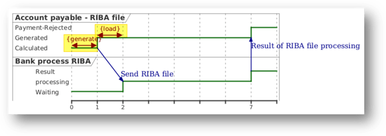
Let’s look at an example. In D365FO, a user generates a RIBA payment file to send to the bank. After processing, the bank returns a response file containing the result of the collection/payment (accepted or protested):

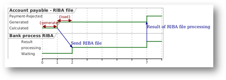
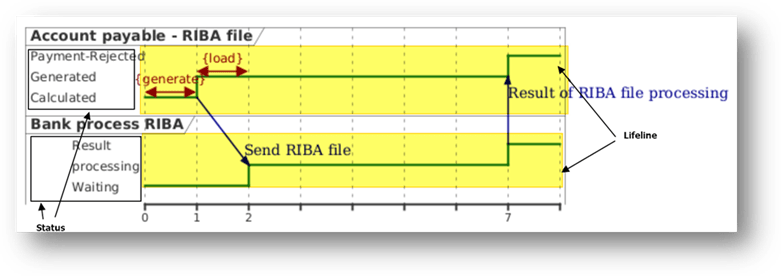
The lifeline represents the solution component that is the focus of our observation. During the process, we observe the evolution of the state changes (or condition changes) for each lifeline over time.

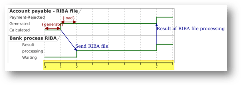
At the bottom, we find the time axis of the observation. In our case, time is expressed in days.

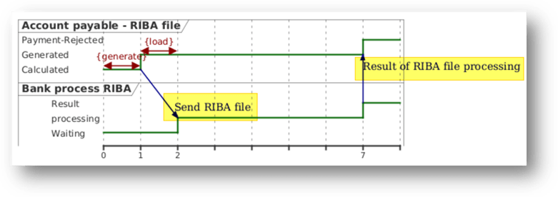
Between the lifelines, there can be communications (messages exchanged between components).

Duration constraints indicate how much time an activity or a specific state is expected to take (or must take).

PlantUml code

For reference, here is the PlantUML code used to generate the diagram (note: this is the same from the code used for the component diagram).

@startuml
robust "Account payable - RIBA file" as D365FO
robust "Bank process RIBA" as BANK
' Duration constraints 
D365FO@0 <-> @1 : {generate}
D365FO@1 <-> @2 : {load}
' Comunication
D365FO@1 -> BANK@2 : Send RIBA file
BANK@7 -> D365FO@7: Result of RIBA file processing
' Status change
@0
D365FO is Calculated
BANK is Waiting 
@1
D365FO is Generated 
@2
BANK is processing
@7
D365FO is Payment-Rejected 
BANK is Result 
@enduml